

Absolute Value Graph Parent Function
| Basic Parent Functions | Writing Transformed Equations from Graphs |
| Generic Transformations of Functions | Rotational Transformations |
| Vertical Transformations | Transformations of Inverse Functions |
| Horizontal Transformations | Applications of Parent Role Transformations |
| Mixed Transformations | More than Practice |
| Transformations Using Functional Annotation |
For Accented Value Transformations, come across theAbsolute Value Transformations section. Here are links to Parent Function Transformations in other sections: Transformations of Quadratic Functions (quick and easy way);Transformations of Radical Functions;Transformations of Rational Functions; Transformations of Exponential Functions;Transformations of Logarithmic Functions; Transformations of Piecewise Functions; Transformations of Trigonometric Functions; Transformations of Inverse Trigonometric Functions
You may non be familiar with all the functions and characteristics in the tables; hither are some topics to review:
- Whether functions are fifty-fifty, odd, or neither, discussed here in the Advanced Functions: Compositions, Even and Odd, and Extrema.
- End behavior and asymptotes, discussed in the Asymptotes and Graphing Rational Functions and Graphing Polynomials sections
- Exponential and Logarithmic Functions
- Trigonometric Functions
Bones Parent Functions
Y'all'll probably study some "popular" parent functions and work with these to larn how to transform functions – how to motility and/or resize them. We call these basic functions "parent" functions since they are the simplest form of that blazon of function, meaning they are as close as they tin get to the origin \(\left( {0,0} \right)\).
The chart below provides some basic parent functions that yous should be familiar with. I've also included the significant points, or critical points, the points with which to graph the parent role. I also sometimes phone call these the "reference points" or "anchor points".
Know the shapes of these parent functions well! Even when using t -charts, y'all must know the general shape of the parent functions in order to know how to transform them correctly!
| Parent Function | Graph | Parent Function | Graph |
| \(y=x\) Domain: \(\left( {-\infty ,\infty } \right)\) End Behavior**: Critical points: \(\displaystyle \left( {-1,-ane} \right),\,\left( {0,0} \correct),\,\left( {one,1} \right)\) |  | \(y=\left| 10 \right|\) Domain: \(\left( {-\infty ,\infty } \right)\) Terminate Behavior: Critical points: \(\displaystyle \left( {-1,1} \right),\,\left( {0,0} \right),\,\left( {one,1} \right)\) |  |
| \(y={{x}^{ii}}\) Domain: \(\left( {-\infty ,\infty } \right)\) End Behavior: Disquisitional points: \(\displaystyle \left( {-i,i} \correct),\,\left( {0,0} \right),\,\left( {one,ane} \right)\) |  | \(y=\sqrt{x}\) Domain: \(\left[ {0,\infty } \right)\) Terminate Behavior: \(\displaystyle \begin{array}{l}x\to 0,\,\,\,\,y\to 0\\ten\to \infty \text{,}\,\,y\to \infty \cease{array}\) Critical points: \(\displaystyle \left( {0,0} \right),\,\left( {1,one} \right),\,\left( {iv,2} \right)\) |  |
| \(y={{x}^{iii}}\) Domain: \(\left( {-\infty ,\infty } \right)\) End Behavior: Disquisitional points: \(\displaystyle \left( {-ane,-ane} \right),\,\left( {0,0} \right),\,\left( {1,1} \right)\) |  | \(y=\sqrt[3]{x}\) Domain: \(\left( {-\infty ,\infty } \right)\) End Behavior: Critical points: \(\displaystyle \left( {-1,-1} \right),\,\left( {0,0} \right),\,\left( {1,1} \right)\) |  |
| \(\begin{assortment}{c}y={{b}^{x}},\,\,\,b>ane\,\\(\text{Example:}\,\,y={{ii}^{x}})\stop{array}\) Exponential, Neither Domain: \(\left( {-\infty ,\infty } \right)\) End Behavior: Critical points: \(\displaystyle \left( {-1,\frac{1}{b}} \right),\,\left( {0,one} \right),\,\left( {1,b} \right)\) Asymptote: \(y=0\) |  | \(\begin{assortment}{c}y={{\log }_{b}}\left( 10 \right),\,\,b>ane\,\,\,\\(\text{Example:}\,\,y={{\log }_{2}}ten)\end{array}\) Log, Neither Domain: \(\left( {0,\infty } \right)\) Terminate Behavior: Disquisitional points: \(\displaystyle \left( {\frac{one}{b},-1} \right),\,\left( {ane,0} \right),\,\left( {b,1} \correct)\) Asymptote: \(ten=0\) |  |
| \(\displaystyle y=\frac{1}{10}\) Rational (Inverse), Odd Domain: \(\left( {-\infty ,0} \right)\cup \left( {0,\infty } \right)\) End Beliefs: Critical points: \(\displaystyle \left( {-1,-1} \right),\,\left( {i,ane} \right)\) Asymptotes: \(y=0,\,\,x=0\) **Annotation that this function is the inverse of itself! |  | \(\displaystyle y=\frac{ane}{{{{10}^{2}}}}\) Rational (Inverse Squared), Even Domain: \(\left( {-\infty ,0} \right)\cup \left( {0,\infty } \right)\) End Behavior: Disquisitional points: \(\displaystyle \left( {-1,\,1} \right),\left( {1,1} \right)\) Asymptotes: \(ten=0,\,\,y=0\) |  |
| \(y=\text{int}\left( x \right)=\left\lfloor x \right\rfloor \) Greatest Integer* , Neither Domain: \(\left( {-\infty ,\infty } \correct)\) Cease Behavior: Disquisitional points: \(\displaystyle \begin{array}{fifty}x:\left[ {-1,0} \right)\,\,\,y:-i\\ten:\left[ {0,ane} \right)\,\,\,y:0\\x:\left[ {one,2} \correct)\,\,\,y:1\end{array}\) |  | \(y=C\) (\(y=2\)) Constant, Even Domain: \(\left( {-\infty ,\infty } \right)\) End Behavior: Critical points: \(\displaystyle \left( {-1,C} \correct),\,\left( {0,C} \right),\,\left( {1,C} \right)\) | |

*The Greatest Integer Function, sometimes chosen the Footstep Function, returns the greatest integer less than or equal to a number (recall of rounding down to an integer). In that location's also a Least Integer Office, indicated by \(y=\left\lceil x \correct\rceil \), which returns the least integer greater than or equal to a number (think of rounding upwardly to an integer).
**Notes on End Behavior: To get thecease beliefs of a part, we only look at thesmallest andlargest values of \(x\), and see which way the \(y\) is going. Not all functions have end beliefs divers; for instance, those that become back and forth with the \(y\) values (called "periodic functions") don't have end behaviors.
Most of the time, our end behavior looks something like this: \(\displaystyle \brainstorm{assortment}{50}10\to -\infty \text{, }\,y\to \,\,?\\ten\to \infty \text{, }\,\,\,y\to \,\,?\end{assortment}\) and we have to make full in the \(y\) part. For example, the end behavior for a line with a positive slope is: \(\begin{assortment}{l}x\to -\infty \text{, }\,y\to -\infty \\x\to \infty \text{, }\,\,\,y\to \infty \cease{array}\), and the end behavior for a line with a negative slope is: \(\begin{array}{l}x\to -\infty \text{, }\,y\to \infty \\x\to \infty \text{, }\,\,\,y\to -\infty \cease{array}\). 1 way to recollect of cease behavior is that for \(\displaystyle x\to -\infty \), we look at what's going on with the \(y\) on the left-hand side of the graph, and for \(\displaystyle x\to \infty \), we look at what's happening with \(y\) on the right-hand side of the graph.
In that location are a couple of exceptions; for example, sometimes the \(x\) starts at 0 (such as in theradical function), nosotros don't accept the negative portion of the \(x\) terminate behavior. Also, when \(x\) starts very shut to 0 (such every bit in in thelog office), nosotros indicate that \(x\) is starting from the positive (right) side of 0 (and the \(y\) is going down); we indicate this past \(\displaystyle x\to {{0}^{+}}\text{, }\,y\to -\infty \).
Generic Transformations of Functions
Again, the "parent functions" assume that we have the simplest form of the function; in other words, the office either goes through the origin \(\left( {0,0} \correct)\), or if it doesn't go through the origin, it isn't shifted in any way. When a office is shifted, stretched (or compressed), or flipped in any way from its "parent function", it is said to be transformed, and is a transformation of a office.
T-charts are extremely useful tools when dealing with transformations of functions. For example, if you know that the quadratic parent part \(y={{x}^{2}}\) is existence transformed two units to the right, and 1 unit down (merely a shift, not a stretch or a flip), nosotros tin can create the original t -chart, following by the transformation points on the exterior of the original points. Then we can plot the "outside" (new) points to get the newly transformed function:
| Transformation | T-chart | Graph | ||||||||
| Quadratic Function \(y={{ten}^{two}}\) Transform office 2 units to the correct, and 1 unit downwards. This turns into the function \(y={{\left( {x-two} \right)}^{2}}-1\), oddly enough! |
Transformed: Domain: \(\left( {-\infty ,\infty } \right)\) Range: \(\left[ {-1,\,\,\infty } \right)\) | |
When looking at the equation of the transformed function, however, we have to be conscientious. When functions are transformed on the outside of the \(f(ten)\) part, you move the function up and down and do the "regular" math, as we'll see in the examples beneath. These are vertical transformations or translations, and affect the \(y\) part of the function. When transformations are made on the inside of the \(f(x)\) part, you move the function back and forth (but practice the "reverse" math – since if you were to isolate the \(10\), you'd motion everything to the other side). These are horizontal transformations or translations, and bear on the \(x\) part of the function.
There are several ways to perform transformations of parent functions; I like to apply t -charts , since they piece of work consistently with ever function. And annotation that in most t-charts, I've included more than just the critical points above, just to show the graphs better.
Vertical Transformations
Hither are the rules and examples of when functions are transformed on the "outside" (find that the \(y\)values are affected). The t-charts include the points (ordered pairs) of the original parent functions, and also the transformed or shifted points. The get-go two transformations are translations, the third is a dilation, and the last are forms of reflections. Accented value transformations will be discussed more expensively in the Accented Value Transformations section!
| Trans formation | What It Does | Example | Graph | ||||||||
| \(f\left( x \right)+b\) Translation | Move graph upwardly \(b\) units Every point on the graph is shifted up \(b\) units. The \(x\)'s stay the aforementioned; add \(b\) to the \(y\) values. | Parent: \(y={{x}^{2}}\) Transformed: \(y={{x}^{ii}}+ \,2\)
| Domain: \(\left( {-\infty ,\infty } \correct)\) Range: \(\left[ {ii,\infty } \correct)\) | ||||||||
| \(f\left( x \right)-b\) Translation | Move graph down \(b\) units Every indicate on the graph is shifted down \(b\) units. The \(x\)'south stay the same; subtract \(b\) from the \(y\) values. | Parent: \(y=\sqrt{x}\) Transformed: \(y=\sqrt{x}- \,3\)
| | ||||||||
| \(a\,\cdot f\left( 10 \right)\) Dilation | Stretch graph vertically by a scale factor of \(a\) (sometimes called a dilation). Notation that if \(a<one\), the graph is compressed or shrunk. Every point on the graph is stretched \(a\) units. The \(x\)'due south stay the same; multiply the \(y\) values by \(a\). | Parent: \(y={{x}^{3}}\) Transformed: \(y={{4x}^{3}}\)
| | ||||||||
| \(-f\left( ten \right)\) Reflection | Flip graph around the \(x\)-axis. Every point on the graph is flipped vertically. The \(x\)'s stay the same; multiply the \(y\) values by \(-1\). | Parent: \(y=\left| x \right|\) Transformed: \(y=-\left| x \right|\)
| | ||||||||
| \(\left| {f\left( ten \right)} \right|\) Absolute Value on the \(y\) (More examples hither in the Absolute Value Transformation section) | Reflect part of graph underneath the \(x\)-centrality (negative \(y\)'s) beyond the \(x\)-centrality. Leave positive \(y\)'s the aforementioned. The \(x\)'southward stay the aforementioned; have the absolute value of the \(y\)'s. | Parent: \(y=\sqrt[3]{10}\) Transformed: \(y=\left| {\sqrt[3]{10}} \right|\)
|  Domain: \(\left( {-\infty ,\infty } \right)\) Range:\(\left[ {0,\infty } \right)\) Domain: \(\left( {-\infty ,\infty } \right)\) Range:\(\left[ {0,\infty } \right)\) |
Horizontal Transformations
Here are the rules and examples of when functions are transformed on the "within" (detect that the \(x\)-values are affected). Notice that when the \(10\)-values are affected, yous practise the math in the "opposite" fashion from what the function looks similar: if you lot're adding on the inside, you decrease from the \(ten\); if you're subtracting on the inside, you add to the \(x\); if you're multiplying on the inside, you dissever from the \(x\); if you're dividing on the inside, y'all multiply to the \(x\). If yous have a negative value on the inside, you lot flip across the \(\boldsymbol{y}\) axis (notice that you nevertheless multiply the \(x\) by \(-1\) only like you practice for with the \(y\) for vertical flips). The first two transformations are translations, the 3rd is a dilation, and the concluding are forms of reflections.
Absolute value transformations will be discussed more than expensively in the Absolute Value Transformations section!
(You may observe it interesting is that a vertical stretch behaves the same way as a horizontal compression, and vice versa, since when stretch something upwardly, nosotros are making it skinnier.)
| Trans formation | What Information technology Does | Example | Graph | ||||||||||||
| \(f\left( {x+b} \correct)\) Translation | Move graph left \(b\) units (Do the "opposite" when change is inside the parentheses or underneath radical sign.) Every signal on the graph is shifted left \(b\) units. The \(y\)'s stay the same; subtract \(b\) from the \(ten\) values. | Parent: \(y={{x}^{2}}\) Transformed: \(y={{\left( {x+2} \right)}^{2}}\)
| | ||||||||||||
| \(f\left( {x-b} \right)\) Translation | Movement graph right \(b\) units Every bespeak on the graph is shifted right \(b\) units. The \(y\)'south stay the same; add together \(b\) to the \(10\) values. | Parent: \(y=\sqrt{10}\) Transformed: \(y=\sqrt{{x- \,3}}\)
| | ||||||||||||
| \(f\left( {a\cdot 10} \right)\) Dialation | Compress graph horizontally by a scale cistron of \(a\) units (stretch or multiply by \(\displaystyle \frac{one}{a}\)) Every point on the graph is compressed \(a\) units horizontally. The \(y\)'s stay the same; multiply the \(x\)-values by \(\displaystyle \frac{1}{a}\). | Parent: \(y={{ten}^{3}}\) T ransformed: \(y={{\left( {4x} \right)}^{3}}\)
| | ||||||||||||
| \(f\left( {-10} \right)\) Reflection | Flip graph around the \(y\)-axis Every point on the graph is flipped around the \(y\) axis. The \(y\)'s stay the same; multiply the \(x\)-values by \(-ane\). | Parent: \(y=\sqrt{10}\) Transformed: \(y=\sqrt{{-10}}\)
| | ||||||||||||
| \(f\left( {\left| x \right|} \right)\) Accented Value on the \(x\) (More than examples here in the Absolute Value Transformation department) | "Throw away" the negative \(x\)'s; reflect the positive \(10\)'s across the \(y\)-centrality. The positive \(10\)'south stay the aforementioned; the negative \(10\)'southward have on the \(y\)'s of the positive \(x\)'s. | Parent: \(y=\sqrt{x}\) Transformed: \(y=\sqrt{{\left| x \right|}}\)
|  Domain: \(\left( {-\infty ,\infty } \right)\)Range:\(\left[ {0,\infty } \right)\) |
Mixed Transformations
Most of the bug you'll become will involve mixed transformations, or multiple transformations, and nosotros practice need to worry about the order in which we perform the transformations. It usually doesn't matter if we make the \(x\) changes or the \(y\) changes offset, but inside the \(ten\)'due south and \(y\)'s, nosotros need to perform the transformations in the order below. Notation that this is sort of similar to the lodge with PEMDAS(parentheses, exponents, multiplication/partition, and addition/subtraction). When performing these rules, the coefficients of the inside \(x\) must exist one ; for example, we would need to have \(y={{\left( {4\left( {x+2} \right)} \right)}^{2}}\) instead of \(y={{\left( {4x+8} \right)}^{2}}\) (by factoring). If you didn't learn it this way, see IMPORTANT NOTE beneath.
Here is the order. We can do steps i and 2 together (order doesn't actually thing), since we can think of the kickoff 2 steps as a "negative stretch/compression."
- Perform Flipping across the axes start (negative signs).
- Perform Stretching and Shrinking next (multiplying and dividing).
- Perform Horizontal and Vertical shifts last (adding and subtracting).
I like to take the disquisitional points and maybe a few more than points of the parent functions, and perform all thetransformations at the same fourth dimension with a t-chart! We just do the multiplication/sectionalization first on the \(x\) or \(y\) points, followed past addition/subtraction. It makes it much easier!Note again that since we don't have an \(\boldsymbol {x}\) "by itself" (coefficient of 1) on the inside, we have to get information technology that manner by factoring! For example,we'd take to change \(y={{\left( {4x+viii} \right)}^{2}}\text{ to }y={{\left( {4\left( {x+two} \right)} \right)}^{two}}\).
Let's try to graph this "complicated" equation and I'll show yous how easy it is to do with a t-nautical chart: \(\displaystyle f(x)=-3{{\left( {2x+eight} \right)}^{ii}}+ten\). (Note that for this example, nosotros could movement the \({{2}^{two}}\) to the outside to get a vertical stretch of \(3\left( {{{ii}^{2}}} \right)=12\), merely nosotros tin't do that for many functions.) We first need to get the \(x\) by itself on the inside by factoring, so we can perform the horizontal translations. This is what we end upward with: \(\displaystyle f(x)=-three{{\left( {2\left( {x+4} \correct)} \right)}^{2}}+10\). Look at what's done on the "exterior" (for the \(y\)'s) and brand all the moves at once, by following the exact math. And so look at what nosotros do on the "inside" (for the \(x\)'s) and brand all the moves at once, merely do the opposite math. We do this with a t -chart.
Start with the parent function \(f(x)={{ten}^{ii}}\). If we look at what we're doing on the outside of what is being squared, which is the \(\displaystyle \left( {2\left( {x+four} \right)} \right)\), we're flipping information technology across the \(x\)-axis (the minus sign), stretching information technology by a factor of 3 , and calculation 10 (shifting upwards 10 ). These are the things that we are doing vertically, or to the \(y\). If we await at what we are doing on the within of what we're squaring, nosotros're multiplying it by 2 , which ways nosotros have to divide by 2 (horizontal compression by a factor of \(\displaystyle \frac{1}{2}\)), and we're adding 4 , which means we have to subtract 4 (a left shift of 4 ). Remember that we do the opposite when we're dealing with the \(10\). Also remember that we e'er have to exercise the multiplication or division first with our points, and so the adding and subtracting (sort of like PEMDAS).
Here is the t-chart with the original function, and and so the transformations on the outsides. Now nosotros tin can graph the outside points (points that aren't crossed out) to get the graph of the transformation. I've also included an explanation of how to transform this parabola without a t-chart, every bit we did in the hither in the Introduction to Quadratics section.
| t-chart | Transformed Graph | ||||||||||||
| Parent: \(y={{x}^{2}}\) (Quadratic) Transformed:\(\displaystyle f(ten)=-3{{\left( {2\left( {10+4} \right)} \right)}^{2}}+10\) y changes:\(\displaystyle f(x)=\color{blue}{{-3}}{{\left( {2\left( {x+4} \right)} \right)}^{2}}\color{blue}{+x}\) 10 changes: \(\displaystyle f(x)=-3{{\left( {\colour{blue}{two}\left( {x\text{ }\color{blue}{{+\text{ }4}}} \correct)} \right)}^{2}}+x\) Opposite for \(x\), "regular" for \(y\), multiplying/dividing first: Coordinate Rule: \(\left( {10,\,y} \right)\to \left( {.5x-4,-3y+10} \correct)\)
| Domain: \(\left( {-\infty ,\infty } \right)\) Range: \(\left( {-\infty ,ten} \correct]\) | ||||||||||||
| How to graphwithout a t-nautical chart: \(\displaystyle f(10)=-three{{\left( {2\left( {x+four} \right)} \right)}^{2}}+10\) Since this is a parabola and information technology's in vertex form (\(y=a{{\left( {x-h} \right)}^{two}}+k,\,\,\left( {h,k} \correct)\,\text{vertex}\)), the vertex of the transformation is \(\left( {-iv,x} \correct)\). Notice that the coefficient of is –12 (by moving the \({{2}^{2}}\) outside and multiplying it by the –3 ). Then the vertical stretch is 12 , and the parabola faces downwards considering of the negative sign. The parent graph quadratic goes upwards 1 and over (and back) i to get 2 more than points, only with a vertical stretch of 12 , we go over (and back) 1 and downward 12 from the vertex. At present we have 2 points from which y'all tin can draw the parabola from the vertex. | |||||||||||||
IMPORTANT Annotation:In some books, for \(\displaystyle f\left( 10 \correct)=-3{{\left( {2x+8} \right)}^{two}}+10\) , they may NOT have you factor out the2 on the inside, but just switch the order of the transformation on the \(\boldsymbol{x}\).
In this case, the guild of transformations would be horizontal shifts, horizontal reflections/stretches, vertical reflections/stretches, and and then vertical shifts. For example, for this problem, y'all would move to the left eight showtime for the \(\boldsymbol{x}\), so compress with a gene of \(\displaystyle \frac {one}{2}\) for the \(\boldsymbol{x}\) (which is opposite of PEMDAS). And then you would perform the \(\boldsymbol{y}\) (vertical) changes the regular way: reverberate and stretch by 3 kickoff, and then shift upward 10. Then, you would have \(\displaystyle {\left( {x,\,y} \right)\to \left( {\frac{i}{2}\left( {ten-8} \right),-3y+10} \correct)}\). Try a t-chart; you'll get the same t-nautical chart as to a higher place!
More Examples of Mixed Transformations:
Here are a couple more examples (using t -charts), with different parent functions. Don't worry if you are totally lost with the exponential and log functions; they will be discussed in the Exponential Functions and Logarithmic Functions sections. Also, the last blazon of function is a rational function that volition be discussed in the Rational Functions section.
| Transformation | T-chart/Domain and Range | Graph | ||||||||
| \(\displaystyle y=\frac{3}{2}{{\left( {-x} \right)}^{3}}+two\) Parent office: \(y={{x}^{three}}\) For this function, notation that could have besides put the negative sign on the outside (thus affecting the \(y\)), and we would have gotten the same graph. |
Domain: \(\left( {-\infty ,\infty } \right)\) Range:\(\left( {-\infty ,\infty } \correct)\) | | ||||||||
| \(\displaystyle y=\frac{i}{two}\sqrt{{-ten}}\) Parent function: \(y=\sqrt{10}\) |
Domain: \(\left( {-\infty ,0} \correct]\) Range:\(\left[ {0,\infty } \correct)\) | | ||||||||
| \(y={{2}^{{x-4}}}+iii\) Parent function: \(y={{2}^{10}}\) For exponential functions, apply –1 , 0 , and 1 for the \(10\)-values for the parent function. (Piece of cake style to think: exponent is like \(x\)). |
Domain: \(\left( {-\infty ,\infty } \right)\) Range:\(\left( {3,\infty } \correct)\) Asymptote: \(y=3\) | | ||||||||
| \(\begin{array}{l}y=\log \left( {2x-ii} \right)-one\\y=\log \left( {2\left( {ten-1} \right)} \right)-one\end{array}\) Parent part: \(y=\log \left( 10 \right)={{\log }_{{x}}}\left( x \correct)\) For log and ln functions, utilize – 1 , 0 , and 1 for the \(y\)-values for the parent part For example, for \(y={{\log }_{3}}\left( {two\left( {x-1} \right)} \right)-1\), the \(x\) values for the parent office would be \(\displaystyle \frac{1}{3},\,one,\,\text{and}\,iii\).) |
Domain: \(\left( {1,\infty } \right)\) Range:\(\left( {-\infty ,\infty } \right)\) Asymptote: \(x=1\) | | ||||||||
| \(\displaystyle y=\frac{3}{{2-10}}\,\,\,\,\,\,\,\,\,\,\,y=\frac{three}{{-\left( {x-2} \right)}}\) Parent part: \(\displaystyle y=\frac{one}{x}\) For this office, notation that could have also put the negative sign on the outside (thus, used \(x+2\) and \(-3y\)). |
Domain:\(\left( {-\infty ,2} \right)\cup \left( {ii,\infty } \right)\) Range:\(\left( {-\infty ,0} \correct)\cup \left( {0,\infty } \correct)\) Asymptotes: \(y=0\) and \(x=2\) | |
Hither's a mixed transformation with the Greatest Integer Function (sometimes called the Floor Role). Note how we can utilise intervals as the \(x\) values to make the transformed part easier to draw:
| Transformation | T-chart/Domain and Range | Graph | ||||||||||||
| \(\displaystyle y=\left[ {\frac{ane}{two}x-2} \correct]+3\) \(\displaystyle y=\left[ {\frac{1}{2}\left( {10-iv} \right)} \right]+3\) Parent function: \(y=\left[ x \right]\) Note how we had to take out the \(\displaystyle \frac{i}{ii}\) to make information technology in the correct class. |
Domain:\(\left( {-\infty ,\infty } \right)\) Range:\(\{y:y\in \mathbb{Z}\}\text{ (integers)}\) | |
Transformations Using Functional Notation
You lot might see mixed transformations in the form \(\displaystyle g\left( x \right)=a\cdot f\left( {\left( {\frac{1}{b}} \correct)\left( {x-h} \right)} \right)+thou\), where \(a\) is the vertical stretch, \(b\) is the horizontal stretch, \(h\) is the horizontal shift to the right, and \(k\) is the vertical shift upwards. In this case, we have the coordinate rule \(\displaystyle \left( {x,y} \right)\to \left( {bx+h,\,ay+m} \right)\). For case, for the transformation \(\displaystyle f(x)=-iii{{\left( {2\left( {x+iv} \correct)} \correct)}^{2}}+10\), we have \(a=-3\), \(\displaystyle b=\frac{one}{2}\,\,\text{or}\,\,.five\), \(h=-four\), and \(1000=10\). Our transformation \(\displaystyle g\left( x \correct)=-3f\left( {2\left( {x+4} \right)} \right)+ten=grand\left( 10 \right)=-3f\left( {\left( {\frac{1}{{\frac{1}{2}}}} \right)\left( {x-\left( {-iv} \right)} \right)} \correct)+ten\) would effect in a coordinate rule of \({\left( {x,\,y} \right)\to \left( {.5x-4,-3y+10} \right)}\). (You may also see this as \(g\left( x \right)=a\cdot f\left( {b\left( {ten-h} \right)} \right)+k\), with coordinate rule \(\displaystyle \left( {x,\,y} \correct)\to \left( {\frac{1}{b}x+h,\,ay+k} \right)\); the end result will be the same.)
Y'all may be given a random point and give the transformed coordinates for the point of the graph. For example, if the betoken \(\left( {8,-2} \correct)\) is on the graph \(y=g\left( ten \right)\), give the transformed coordinates for the point on the graph \(y=-6g\left( {-2x} \correct)-2\). To do this, to get the transformed \(y\), multiply the \(y\) part of the point past –6 and then subtract 2 . To get the transformed \(x\), multiply the \(10\) role of the point by \(\displaystyle -\frac{1}{2}\) (contrary math). The new bespeak is \(\left( {-4,10} \right)\). Let's exercise another case: If the betoken \(\left( {-iv,1} \correct)\) is on the graph \(y=g\left( x \right)\), the transformed coordinates for the point on the graph of \(\displaystyle y=2g\left( {-3x-2} \right)+3=2g\left( {-three\left( {x+\frac{2}{iii}} \right)} \right)+3\) is \(\displaystyle \left( {-4,1} \correct)\to \left( {-4\left( {-\frac{1}{3}} \right)-\frac{2}{3},2\left( 1 \right)+iii} \right)=\left( {\frac{2}{3},5} \right)\) (using coordinate rules \(\displaystyle \left( {x,\,y} \right)\to \left( {\frac{1}{b}x+h,\,\,ay+k} \right)=\left( {-\frac{1}{3}x-\frac{2}{iii},\,\,2y+3} \correct)\)).
You may also be asked to transform a parent or non-parent equation to become a new equation. We can do this without using a t-chart, but by using substitution and algebra. For example, if nosotros want to transform \(f\left( x \right)={{x}^{2}}+4\) using the transformation \(\displaystyle -2f\left( {x-1} \right)+3\), we tin can but substitute "\(x-1\)" for "\(x\)" in the original equation, multiply by –2 , and so add 3 . For example: \(\displaystyle -2f\left( {x-one} \right)+3=-two\left[ {{{{\left( {10-1} \correct)}}^{2}}+four} \right]+3=-2\left( {{{x}^{2}}-2x+1+4} \right)+three=-2{{x}^{2}}+4x-7\). We used this method to help transform a piecewise office here.
Transformations in Function Note (based on Graph and/or Points).
You may too be asked to perform a transformation of a part using a graph and individual points; in this instance, y'all'll probably be given the transformation in function notation. Note that we may demand to utilize several points from the graph and "transform" them, to make sure that the transformed role has the right "shape".
Here are some examples; the second instance is the transformation with an absolute value on the \(ten\); see the Absolute Value Transformations section for more item.
| Original Graph and Points of Function | Transformation Example | Transformation Example | ||||||||||||||||||||
| Original Function: Domain: \(\left[ {-4,v} \correct]\) Range: \(\left[ {-seven,5} \right]\) Key Points:
Remember to describe the points in the aforementioned order as the original to make it easier! If you're having problem drawing the graph from the transformed ordered pairs, only take more points from the original graph to map to the new one! | Transformation:\(\displaystyle f\left( {-\frac{1}{ii}\left( {x-one} \correct)} \correct)-3\) \(y\) changes:\(\displaystyle f\left( {-\frac{1}{2}\left( {ten-ane} \right)} \right)\color{blueish}{{-\text{ }3}}\) \(10\) changes:\(\displaystyle f\left( {\colour{blue}{{-\frac{1}{2}}}\left( {x\text{ }\color{blue}{{-\text{ }1}}} \correct)} \right)-3\) Notation that this transformation flips effectually the \(\boldsymbol{y}\)– centrality, has a horizontal stretch of 2 , moves right by 1 , anddownward past 3 . Key Points Transformed: (we practice the "reverse" math with the "\(x\)")
Transformed Function: Domain: \(\left[ {-9,nine} \right]\) Range: \(\left[ {-x,2} \right]\) | Transformation: \(\displaystyle f\left( {\left| x \right|+1} \right)-2\) \(y\) changes: \(\displaystyle f\left( {\left| x \right|+1} \correct)\colour{blue}{{\underline{{-\text{ }2}}}}\) \(10\) changes:\(\displaystyle f\left( {\color{blue}{{\underline{{\left| x \right|+1}}}}} \correct)-2\): Annotation that this transformation moves down past 2 , and left ane . Then, for the within accented value, nosotros will "get rid of" any values to the left of the \(y\)-axis and replace with values to the right of the \(y\)-axis, to make the graph symmetrical with the \(y\)-axis. Nosotros do the absolute value function terminal, since information technology's but effectually the \(x\) on the within. Let's just exercise this one via graphs. First, move down 2 , and left 1 : And then reflect the right-hand side across the \(y\)-axis to make symmetrical. Transformed Function: Domain: \(\left[ {-4,4} \right]\) Range:\(\left[ {-9,0} \right]\) |

Writing Transformed Equations from Graphs
You might be asked to write a transformed equation, requite a graph. A lot of times, you can simply tell by looking at it, but sometimes yous have to employ a point or two. And y'all do have to be careful and check your work, since the social club of the transformations tin thing.
Note that when figuring out the transformations from a graph, it's difficult to know whether you have an "\(a\)" (vertical stretch) or a "\(b\)" (horizontal stretch) in the equation \(\displaystyle one thousand\left( x \correct)=a\cdot f\left( {\left( {\frac{1}{b}} \right)\left( {x-h} \right)} \right)+k\). Sometimes the problem will indicate what parameters (\(a\), \(b\), and so on) to look for. For others, similar polynomials (such as quadratics and cubics), a vertical stretch mimics a horizontal compression, so it's possible to gene out a coefficient to turn a horizontal stretch/compression to a vertical compression/stretch. (For more complicated graphs, y'all may desire to have several points and perform a regression in your figurer to get the function, if you're allowed to exercise that).
Here are some problems. Note that atransformed equation from an absolute value graph is in the Absolute Value Transformationsdepartment.
| Transformed Graph | Getting Equation |
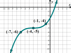
| Write the general equation for the cubic equation in the form: \(\displaystyle y={{\left( {\frac{one}{b}\left( {ten-h} \right)} \right)}^{iii}}+yard\). | We see that that the center point, or critical point is at \(\left( {-4,-five} \right)\), so the cubic is in the form: \(\displaystyle y={{\left( {\frac{i}{b}\left( {x+4} \right)} \correct)}^{three}}-five\). Notice that to get dorsum and over to the next points, nosotros become back/over \(three\) and downwardly/upwards \(1\), so nosotros see there'south a horizontal stretch of \(3\), so \(b=three\). (We could have also used some other indicate on the graph to solve for \(b\)). We accept \(\displaystyle y={{\left( {\frac{1}{3}\left( {x+4} \right)} \right)}^{3}}-5\). Try information technology – information technology works! Note that if nosotros wanted this function in the grade \(\displaystyle y=a{{\left( {\left( {x-h} \right)} \right)}^{3}}+k\), we could use the point \(\left( {-7,-6} \right)\) to become \(\displaystyle y=a{{\left( {\left( {ten+4} \right)} \right)}^{three}}-5;\,\,\,\,-6=a{{\left( {\left( {-7+4} \right)} \correct)}^{3}}-five\), or \(\displaystyle a=\frac{ane}{{27}}\). This makes sense, since if we brought the \(\displaystyle {{\left( {\frac{1}{3}} \right)}^{3}}\) out from in a higher place, information technology would be \(\displaystyle \frac{1}{{27}}\)!) |
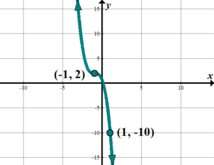
| Notice the equation of this graph in whatsoever form: | Here'due south a generic method you lot can typically employ: We run across that this is a cubicpolynomial graph (parent graph \(y={{ten}^{3}}\)), but flipped around either the \(x\) the \(y\)-axis, since it's an odd function; let's utilize the \(10\)-axis for simplicity's sake. The equation will exist in the form \(y=a{{\left( {x+b} \right)}^{three}}+c\), where \(a\) is negative, and it is shifted upward \(2\), and to the left \(1\). Now nosotros take \(y=a{{\left( {x+one} \right)}^{3}}+2\). We need to find \(a\); apply the point \(\left( {1,-x} \correct)\): \(\begin{align}-10&=a{{\left( {1+1} \right)}^{3}}+two\\-10&=8a+2\\8a&=-12;\,\,a=-\frac{{12}}{8}=-\frac{3}{2}\end{align}\). The equation of the graph is: \(\displaystyle y=-\frac{iii}{2}{{\left( {x+ane} \right)}^{3}}+two\). Exist sure to cheque your answer by graphing or plugging in more points! √ |
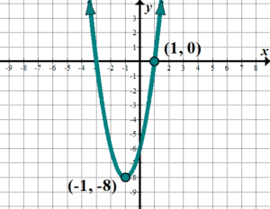
| Discover the equation of this graph in any class: | The graph looks like a quadratic with vertex \(\left( {-ane,-eight} \right)\), which is a shift of \(viii\) down and \(1\) to the left. This will give us an equation of the form \(y=a{{\left( {x+i} \right)}^{two}}-8\), which is (not so coincidentally!) the vertex form for quadratics. We need to find \(a\); use the point \(\left( {1,0} \right)\):\(\begin{marshal}y&=a{{\left( {10+i} \right)}^{2}}-8\\\,0&=a{{\left( {1+1} \right)}^{2}}-eight\\8&=4a;\,\,a=2\end{marshal}\). The equation of the graph so is: \(y=2{{\left( {ten+1} \right)}^{2}}-8\). Note: nosotros could have too noticed that the graph goes over \(1\) and upward \(ii\) from the vertex, instead of over \(ane\) and up \(1\) normally with \(y={{x}^{2}}\). This would mean that our vertical stretch is \(2\). |
| Find the equation of this graph in any form: | The graph looks like a rational with the "centre" of asymptotes at \(\left( {-ii,3} \right)\), which is a shift of 2 to the left and 3 up. This will give us an equation of the form \(\displaystyle y=a\left( {\frac{ane}{{x+2}}} \right)+3\), with asymptotes at \(x=-2\) and \(y=three\). We demand to find \(a\); use the given indicate \((0,iv)\): \(\begin{marshal}y&=a\left( {\frac{1}{{x+2}}} \correct)+three\\4&=a\left( {\frac{1}{{0+two}}} \right)+3\\i&=\frac{a}{2};\,a=2\stop{align}\). The equation of the graph is: \(\displaystyle y=2\left( {\frac{1}{{x+2}}} \right)+3,\,\text{or }y=\frac{2}{{x+2}}+three\). Note: we could take also noticed that the graph goes over one and up 2 from the center of asymptotes, instead of over 1 and up i normally with \(\displaystyle y=\frac{1}{x}\). This would mean that our vertical stretch is 2 . |
| Observe the equation of this graph with a base of \(.five\) and horizontal shift of \(-1\): | Nosotros encounter that thisexponential graph has a horizontal asymptote at \(y=-3\), and with the horizontal shift, we have \(y=a{{\left( {.5} \right)}^{{x+1}}}-three\) so far. When you have a problem like this, first use any betoken that has a " 0 " in it if you can; information technology volition be easiest to solve the arrangement. Solve for \(a\) start using point \(\left( {0,-1} \right)\): \(\begin{array}{c}y=a{{\left( {.5} \right)}^{{x+1}}}-3;\,\,-1=a{{\left( {.5} \right)}^{{0+1}}}-iii;\,\,\,\,2=.5a;\,\,a=4\\y=4{{\left( {.v} \right)}^{{x+1}}}-3\finish{array}\) Note that there are more than examples of exponential transformations here in the Exponential Functions section, and logarithmic transformations hither in the Logarithmic Functions section. |


Rotational Transformations
You may be asked to perform a rotation transformation on a office (you usually see these in Geometry class). A rotation of 90° counterclockwise involves replacing \(\left( {x,y} \correct)\) with \(\left( {-y,10} \right)\), a rotation of 180° counterclockwise involves replacing \(\left( {x,y} \right)\) with \(\left( {-x,-y} \right)\), and a rotation of 270° counterclockwise involves replacing \(\left( {x,y} \correct)\) with \(\left( {y,-x} \right)\). Hither is an example:
| Transformation | Example | Graph | ||||||||||||
| Rotate graph 270° counterclockwise | Parent: \(y={{ten}^{2}}\) Supercede \((x,y)\) with \((y,–ten)\)
| Rotated Function Domain: \(\left[ {0,\infty } \right)\) Range:\(\left( {-\infty ,\infty } \correct)\) |
Transformations of Inverse Functions
We learned virtually Inverse Functions here, and you might be asked to compare original functions and changed functions, every bit far as their transformations are concerned. Remember that an inverse function is ane where the \(ten\) is switched by the \(y\), so the all the transformations originally performed on the \(x\) will be performed on the \(y\):
Problem:
If a cubic function is vertically stretched by a factor of 3 , reflected over the \(\boldsymbol {y}\)-axis, and shifted down two units, what transformations are washed to its inverse role?
Solution:
We demand to practice transformations on the opposite variable. Thus, the inverse of this office volition be horizontally stretched past a factor of 3 , reflected over the \(\boldsymbol {x}\)-axis, and shifted to the left two units. Here is a graph of the two functions:
![]()
Note that examples of Finding Inverses with Restricted Domains can be establish here.
Applications of Parent Function Transformations
You may see a "word problem" that used Parent Function Transformations, and you tin use what y'all know near how to shift a function. Here is an example:
| Transformation Application Problem | Solution |
| The post-obit polynomial graph shows the turn a profit that results from selling math books after September i. The polynomial is \(p\left( x \right)=5{{x}^{iii}}-20{{ten}^{2}}+40x-one\), where \(ten\) is the number of weeks afterwards September 1. The publisher of the math books were one week behind however; depict how this new graph would look and what would exist the new (transformed) function? | Since nosotros're moving the time in weeks by i week, nosotros are shifting the graph horizontally, or shifting the inside, or \(ten\) values. Since our get-go profits volition start a little after week 1 , we can come across that we need to move the graph to the correct. When we motion the \(x\) part to the right, nosotros have the \(x\) values and subtract from them, so the new polynomial will be \(d\left( x \correct)=5{{\left( {x-1} \correct)}^{3}}-20{{\left( {10-1} \right)}^{2}}+40\left( {10-one} \correct)-one\). (I won't multiply and simplify.) Meet how this was much easier, knowing what nosotros know most transforming parent functions? |
Learn these rules, and do, practice, practice!
For Practice: Use the Mathway widget below to try aTransformation trouble. Click on Submit (the bluish pointer to the correct of the problem) and click on Describe the Transformation to run across the answer.
You can also type in your own trouble, or click on the three dots in the upper right hand corner and click on "Examples" to drill down past topic.
If you click on Tap to view steps, or Click Here, you tin annals at Mathway for a gratis trial, and and then upgrade to a paid subscription at any fourth dimension (to go any blazon of math problem solved!).
On to Absolute Value Transformations – yous are ready!

Absolute Value Graph Parent Function,
Source: https://mathhints.com/parent-graphs-and-transformations/
Posted by: waggoneramust1994.blogspot.com
0 Response to "Absolute Value Graph Parent Function"
Post a Comment